Stock Prediction with LSTM Nets
Introduction
In this blogpost I’ve taken inspiration from some parts of my master thesis.
Stock market data is often analyzed in terms of returns, i.e. \((price_t - price_{t-1}) / price_{t-1}\). Financial returns has certain noticable characteristics, some of them are:
- No linear correlation
- Slow decay of linear autocorrelation of absolute returns
- Heavy tails
- Larger tail for losses than for positive returns
- The shape of the distribution is dynamic
- Volatility clustering
- Conditional heavy-tails
- Correlation between trading volume and volatility
One type of models that are successfully used to model financial returns are ARMA-GARCH models. These models have autoregressive properties both in the time series itself (the ARMA part), but also in its variance (the GARCH part). For more info see the wiki page.
Another way to try to capture autoregressive properties in time series data is to use RNNs (recurrent neural networks). LSTM (long short-term memory) networks are able to capture autoregressive properties of arbitrary length and has become very popular lately.
Instead of regular neural network nodes, a LSTM network consists of LSTM blocks. Consider the following system of equations,
\begin{equation} f_t = g \left( W_f \cdot [x_t, h_{t-1}] + b_f \right) \end{equation}
\begin{equation} i_t = g \left( W_i \cdot [x_t, h_{t-1}] + b_i \right) \end{equation}
\begin{equation} o_t = g \left( W_0 \cdot [x_t, h_{t-1}] + b_0 \right) \end{equation}
\begin{equation} c_t = f_t \circ c_{t-1} + i_t \circ tanh \left( W_c \cdot [x_t, h_{t-1}] + b_c \right) \end{equation}
\begin{equation} h_t = o_t \circ tanh \left( c_t \right) \end{equation}
where \(g(\cdot)\) is the sigmoid function, \(tanh(\cdot)\) is the hyperbolic tangent, \(x_t\) is the input vector, \(h_t\) is the output vector, \(c_t\) is a cell state vector. \(W\) are weights and \(b\) are biases. \(f_t\), \(i_t\) and \(o_t\) are called gates of the block. Note that \(\circ\) is not matrix multiplication but the Schur product, i.e. entry wise product.
This system of equations represent one LSTM block. One can see the recurrent properties of the block as \(h_{t-1}\), i.e., the output vector for period \(t-1\), is included in the calculation of the output vector \(h_t\).
The first gate of the LSTM block, \(f_t\) is the forget gate. This gate decided upon which information will be forgotten in the cell state, \(c_t\). Notice how the linear expression is wrapped in a sigmoid function, which indeed is bounded between 0 and 1. If the optimization sets \(f_t\) to 0 the value is forgotten in the calculation. The input gate, \(i_t\), regulates what new information will be stored in the cell state. \(o_t\) is the output gate. The output vector \(h_t\) is a combination of the output gate and the cell state which contains stored information.
The key to understand LSTM network is to understand the activation functions. How these functions can help the blocks store and forget information. The optimization takes care of setting the adjustable parameters accordingly.
A very good blog post that intuitively helps one to understand LSTM’s is Understanding LSTM Networks
LSTM model
3 hidden LSTM layers. The first layer has 4 blocks, the second 50, and the third 100 LSTM blocks. Both the second and the third layer is regularized by a dropout layer (50%). The output layer consists of a softmax classification function, yielding a 2-dimensional vector where the first value indicates the probability that the market has positive return tomorrow, and the second element in the vector indicates the probability that the index has negative return tomorrow.
Empirics
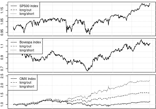
The data set consists of multivariate time series return data from 2009 to 2017 with regards to the US, Brazilian and Swedish stock market index. 33% of the data is saved for testing.
Figure 1: S&P 500, Bovespa, OMX.
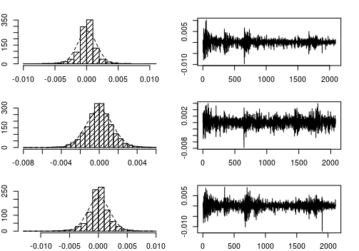
Figure 2: LSTM 1 day ahead forcast output. Black indicates probability of positive returns and grey indicates probability of negative returns.
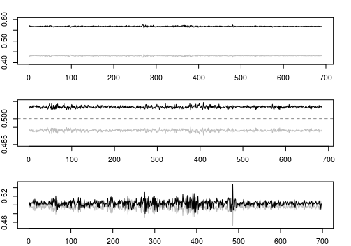
Note: Regarding the US and Brazilian market the model says “always buy”, i.e. the probability of positive returns tomorrow is always over 50%. Looking at the Swedish market, the model seems to have found some structure. Let’s build two trading strategies and evaluate the models generalization.
Figure 3: Trading strategy implemented.
Conclusion
The LSTM model doesn’t find any structure in the US or Brazilian market. However, the model finds some successfull generalization for the Swedish market. Note that this could very well be due to optimization traps etc, but is indeed an interesting result.