ReLU Nets are Splines
Introduction
Artificial Neural Networks has been increasingly popular during the last years. With API’s such as TensorFlow deep learning is easily accessible not only for machine learning experts. This leads to a lot of practice and hands on experience, but it might also lead to a lack of theoretical understanding about the approximation methods.
In this post I will try to shed some light upon how a neural network with the popular ReLU activation function actually makes its approximations.
The theorems and proofs in this blog post are taken from my bachelor’s thesis in mathematics/numerical analysis. When writing the thesis, my coauthor and I got inspiration from Chen 2016.
ReLU nets are linear splines
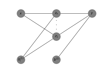
The neural network model that will be investigated has one single hidden layer, with an arbitrary number of nodes, the rectified linear unit as activation function for the hidden layer and the unit function (i.e. \(g(a) = a\)) as activation function for the final output layer. The network maps one input value to one output value. Hence, \(y: \mathbb{R} \rightarrow \mathbb{R}\). Thus the network can be expressed as:
\begin{equation} y = \sum_{i=1}^n w_i^{(2)} z_i + b^{(2)} \tag{1} \end{equation}
where,
\begin{equation} z_i = g(w_i^{(1)}x + b_i^{(1)}) \tag{2} \end{equation}
Figure 1 is showing a visual representation of Equation 1 and 2,
The ReLU function is defined as,
\begin{equation} g(a) \equiv \max(0,a) \tag{3} \end{equation}
Already when looking at the ReLU function one can see that it looks like a linear spline. It has two “line parts” and one discontinuity at 0. By looking at equation 2 one can see how \(z\) is just an affine transformation of the input with a wrapper, i.e. \(g()\). Since \(g()\) is defined as the the ReLU function the hinge will be where the affine transformation is equal to zero.
Solving for where the transformation is equal to zero,
\begin{equation} w_i^{(1)}x + b_i^{(1)} = 0 \Leftrightarrow x = -\frac{b_i^{(1)}}{w_i^{(1)}} \tag{4} \end{equation}
Thus, the knots of the linear spline is defined by the fraction of the weights and biases. This means that the position of the knots of the linear spline is adjusted when the weights and biases are updated, i.e. when the network is optimized/trained.
Upper bound of knots
In fact, one can prove that there is an upper bound on the number of knots produced by the ReLU network’s approximation. When looking at a ReLU net with one hidden layer the number of knots is bounded by the number of nodes in the network. The relationship is \(k \leq n\), where \(k\) is the number of inner knots of the linear spline and \(n\) is the number of nodes of the network. The reason that it can be less is because theoretically two or more knots of the approximation can coincide, however this is not very likely in practice.
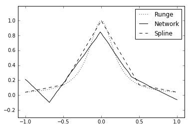
Numerical experiment
In order to investigate this property a one hidden layer network with ReLU activation is set up in Keras with TensorFlow backend and tested on Runge’s function, i.e. \(\frac{1}{1+25x^2}\). The network approximation is compared to a linear spline with equidistant placed knots.
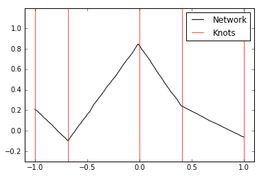
The network approximation plotted below has 3 inner nodes plus 2 endpoints, yielding 5 knots.
Furthermore, the positions of the inner knots are plotted by solving for \(x\), i.e. \(-\frac{b_i^{(1)}}{w_i^{(1)}}\),
Theorems and proofs
In order to show that the ReLU net is a linear spline it is helpful to first define what a linear spline is.
A function, \(S\), is called a linear spline or a spline of degree \(1\) if for a finite set of knots \(x_0,x_1,...,x_n\) the following two conditions hold,
-
on each interval \([x_{i-1},x_i]\), \(S\) is a polynomial of maximal degree \(1\)
-
\(S\) is continuous
Theorem 1:
Let \(y\) be a neural network defined by Equation 1 and 2 with the ReLU activation function defined as in Equation 3. \(y\) is a function \(\mathbb{R} \rightarrow \mathbb{R}\) satisfying the conditions in the definition of the linear spline and is thus a linear spline. The knots are defined by the networks’s weights and biases.
Proof:
Let \(g(a)\) be the ReLU function. \(g(a)\) is a linear spline with knots \(X = \{ a_{min}, 0, a_{max} \}\).
- Let \(z\) be an inner node of the neural network, \(y\), defined as \(z = g(wx + b)\). \(z\) is a linear spline with knots \(X = \{\frac{x_{min} - b}{w}, \frac{-b}{w}, \frac{x_{max} - b}{w} \}\).
- The whole network \(y\) is an affine transformation of the inner nodes \(z_1,z_2,...,z_n\) such that \(y(x) = w^{(2)}_1g(w_1^{(1)} x + b^{(1)}_1) + w^{(2)}_2g(w_2^{(1)} x + b^{(1)}_2) + ... + w^{(2)}_n g(w_n^{(1)} x + b^{(1)}_n) + b^{(2)}\)
By creating the set of knots \(X_y\) for \(y\) as the union of all the knots of the inner network nodes, \(X_1,X_2, ..., X_n\) such that \(X_y = X_1 \cup X_2 \cup ... \cup X_n\). Then \(y\) is defined by a set of knots. As \(y\) consists of a linear combination of \(z_i\)’s the two conditions for linear splines are preserved in \(y\). Combining these results one sees that \(y\) is a linear spline. Q.E.D.
Theorem 2:
The number of inner knots, \(k\), of a spline, \(y\), defined by Equation 1 and 2 with activation function as defined in Equation 3, is bounded by the number of inner network nodes, \(n\). That is, the number of inner spline knots satisfies the relation \(k \leq n\).
Proof:
Writing Equation 1 as \(y = w_1^{(2)} z_1 + w_2^{(2)} z_2 + ... + w_n^{(2)} z_n + b^{(2)}\), where \(z_i\) is defined as in Equation 2. The derivative of \(y\) with regard to \(x\) is, \(y^\prime=w_1^{(2)} z_1^\prime w_1^{(1)} +...+ w_n^{(2)} z_n^\prime w_1n^{(1)}\). The derivative consists of \(n\) terms \(z_1,z_2,...z_n\). The terms can at most be discontinuous at one point. That is when the argument for \(z_i(x)\) is \(x = \frac{-b_i^{(1)}}{w_i^{(1)}}\). Hence, there are at most \(n\) discontinuities in \(y^\prime\).
The relation is \(k \leq n\) due to the fact that two knots can overlap one another if \((\frac{-b_i^{(1)}}{w_i^{(1)}}) = (\frac{-b_j^{(1)}}{w_j^{(1)}})\) for two different network nodes \(z_i\) and \(z_j\). The knots can also lie outside of the range of \([x_{min},x_{max}]\) if \(\frac{-b_i^{(1)}}{w_i^{(1)}} < x_{min}\) or \(\frac{-b_i^{(1)}}{w_i^{(1)}} > x_{max}\). Q.E.D.