Endogeneity

Introduction

This post considers the econometric concept of endogeneity in which the explanatory variable in a regression in correlated with the error term. A short explanation is given, followed by a numerical example in R using instrumental variable (IV) estimation.

Short theory

Consider the OLS estimator,

\begin{equation} \hat{\beta} = (X’X)^{-1}X’y \iff \end{equation}

\begin{equation} \hat{\beta} = (X’X)^{-1}X’(X \beta +u) \iff \end{equation}

\begin{equation} \hat{\beta} = (X’X)^{-1}(X’X) \beta + (X’X)^{-1}X’u \iff \end{equation}

\begin{equation} \hat{\beta} = \beta + (X’X)^{-1}X’u \end{equation}

Thus, in order for the estimator to be unbiased \(\mathbb{E}((X'X)^{-1}X'u)=0\) needs to hold. The standard OLS assumption \(\mathbb{E}(u \mid X)=0\) yields unbiasedness,

\begin{equation} \mathbb{E}(\hat{\beta}) = \beta + \mathbb{E}((X’X)^{-1}X’u) \iff \end{equation}

\begin{equation} \mathbb{E}(\hat{\beta}) = \beta + \mathbb{E}(\mathbb{E}((X’X)^{-1}X’u|X)) \iff \end{equation}

\begin{equation} \mathbb{E}(\hat{\beta}) = \beta + \mathbb{E}((X’X)^{-1}X’ \mathbb{E}(u|X)) \iff \end{equation}

\begin{equation} \mathbb{E}(\hat{\beta}) = \beta \end{equation}

by using the law of iterated expectations. (For consistency this needs to hold asymptotically). This means that if endogeneity is present, i.e. \(X\) is correlated with \(u\), the estimator is biased and inconsistent.

One might note that \((X'X)^{-1}X'u\) is simply another regression. However, what is observed is not \(u\) but \(\hat{u}\) and \(\mathbb{E}(X \hat{u})\) is by construction of the estimator (FOC of OLS / when you minimize the squared errors) equal to \(0\), thus the bias cannot be measured. This can be seen by,

\begin{equation} (X’X)\hat{\beta} = X’y \iff \end{equation}

\begin{equation} (X’X)\hat{\beta} = X’(X \hat{\beta} + \hat{u}) \end{equation}

\begin{equation} (X’X)\hat{\beta} = (X’X)\hat{\beta} + X’\hat{u} \end{equation}

\begin{equation} X’\hat{u} = 0 \end{equation}

This means that the observed correlation between \(X\) and \(\hat{u}\) is \(0\). It also means that the sum of \(\hat{u}\) is equal to \(0\) if we have an intercept in the model, since that represents a column of \(1\)’s in the \(X\) matrix.

The IV estimator

\begin{equation} \hat{\beta} = \frac{(z’z)^{-1}z’y}{(z’z)^{-1}z’x} = (z’x)^{-1}z’y \end{equation}

For more information see e.g. wiki.

Numerical example

\begin{equation} y = 0.5x + u \end{equation}

\begin{equation} x = z + v \end{equation}

where \(z\) is distributed \(\mathcal{N}(2,1)\) and \((u,v)\) are distributed multivariate normal with means \(0\), variances \(1\) and correlation \(0.8\). This means that \(x\) is correlated with \(u\), hence the regression of \(y\) on \(x\) is inconsistent and biased.

The \(z\) variables is an instrument since it is correlated with \(x\) but uncorrelated with \(u\).

We start by defining a linear regression function,

lin_reg <- function(x, y, z = 0, intercept = TRUE, instrument = FALSE){

  x = as.matrix(x)
  y = as.matrix(y)

  output = list()

  if (intercept){
    x = cbind(1,x)
    z = cbind(1,z)
  }

  if (instrument){
    output[['coeffs']] = solve(t(z) %*% x) %*% t(z) %*% y
  } else {
    output[['coeffs']] = solve(t(x) %*% x) %*% t(x) %*% y
  }

  output[['preds']] = x %*% output[['coeffs']]
  output[['resids']] = output[['preds']] - y
  output[['mse']] = mean(output[['resids']]^2)

  return(output)
}

Simulation of data,

library(MASS)

set.seed(42)

z <- rnorm(10000, 2, 1)

sigma <- matrix(data = c(1,0.8,0.8,1), nrow = 2, ncol = 2)
uv <- mvrnorm(n = 10000, mu = c(0,0), Sigma = sigma)

u <- uv[,1]
v <- uv[,2]

x <- z + v
y <- 0.5*x + u

Running the regressions,

reg_xy <- lin_reg(x, y, intercept = TRUE)

The estimated coefficients, where the first element is the intercept and the second element the slope,

> reg_xy[['coeffs']]
           [,1]
[1,] -0.8003143
[2,]  0.8978703

Running the IV estimation,

reg_xzy <- lin_reg(x, y, z, intercept = TRUE, instrument = TRUE)

> reg_xzy[['coeffs']]
          [,1]
[1,] 0.0139782
[2,] 0.4887241

By observing the results the IV estimator is accurate in estimating the true dgp whereas the biased/inconsistent estimator is not.

How does the bias depend on the correlation?

One question that comes to mind is how does the biased/inconsistent estimator perform under different correlations? In the previous example a quite large correlation between \(u\) and \(v\) was imposed.

The following piece of code simulates data from \(0\) correlation between \(u\) and \(v\) to correlation \(1\). Then it plots the coefficients and we can observe how the estimated coefficients change when the correlation increases.

set.seed(42)
z <- rnorm(10000, 2, 1)

coeffs_a<- list()
coeffs_b <- list()

for (i in seq(0, 1, by=0.01)){
  sigma <- matrix(data = c(1, i, i, 1), nrow = 2, ncol = 2)
  uv <- mvrnorm(n = 10000, mu = c(0,0), Sigma = sigma)
  u <- uv[,1]
  v <- uv[,2]

  x <- z + v
  y <- 0.5*x + u

  reg_xy <- lin_reg(x, y, intercept = TRUE)

  coeffs_a[[toString(i)]] <- reg_xy[['coeffs']][1,]
  coeffs_b[[toString(i)]] <- reg_xy[['coeffs']][2,]
}

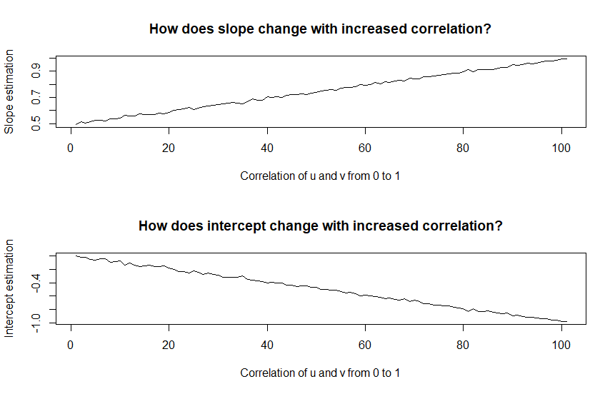
The beta coefficient starts at the true value when the correlation is \(0\) (so does the intercept) and then linearly deviates. If also negative correlation is considered the following results arise,

The linear relationship continues. This seems bad, however what happens if we plot the \(x\) and \(y\) data together with different regression lines corresponding to different correlations? How off are they? To give “less” advantage to the biased/inconsistent regression, I plot simulated data where \(u\) and \(v\) has zero correlation.

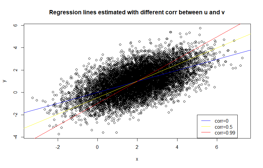
Note that you need to evalute the intercept at \((0,0)\).

Although, the red line with higher bias has a poorer fit it might be an okay approximation depending on the task at hand.

Further, it would of course be interesting to look at the data from the original numerical example (with correlation 0.8) and comapre the inconsistent OLS estimator with the consistent IV estimator. The magnitude of the distortion looked severe when comapring the coefficients, but how does it look visually?

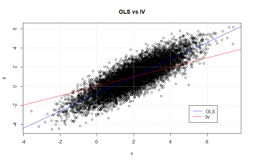
This is actually an extremely interesting figure. Note that it looks like the blue line, i.e. the OLS estimator, represents the data better than the IV estimator. Thus, from a prediction point of view, does the IV estimator add any value?

When is the distortion too much?

When reading econometrics litterature one can come by statements saying that the endogeneity problem can be so severe such that the sign of the slope coefficient is wrong. By looking at,

\begin{equation} \hat{\beta} = \beta + (X’X)^{-1}X’u \end{equation}

one can see that if \(\beta > 0\) but \((X'X)^{-1}X'u << 0\) such that \(\hat{\beta} <0\) then the interpretation of estimated coefficient can be completely misleading.

By simulating the same data as before, with the only changes that \(\beta = 0.1\) instead of \(0.5\) and correlation between \(u\) and \(v\) is \(-0.8\) instead of \(0.8\), lead to the following estimations,

> reg_xy <- lin_reg(x, y, intercept = TRUE)
> reg_xy[['coeffs']]
           [,1]
[1,]  0.7928535
[2,] -0.3007175
>
> reg_xzy <- lin_reg(x, y, z, intercept = TRUE, instrument = TRUE)
> reg_xzy[['coeffs']]
            [,1]
[1,] -0.01634006
[2,]  0.10654534

Here one can see that the OLS estimator is giving a negative slope coefficient while the IV estimator gives an accurate approximation. Plotting this,

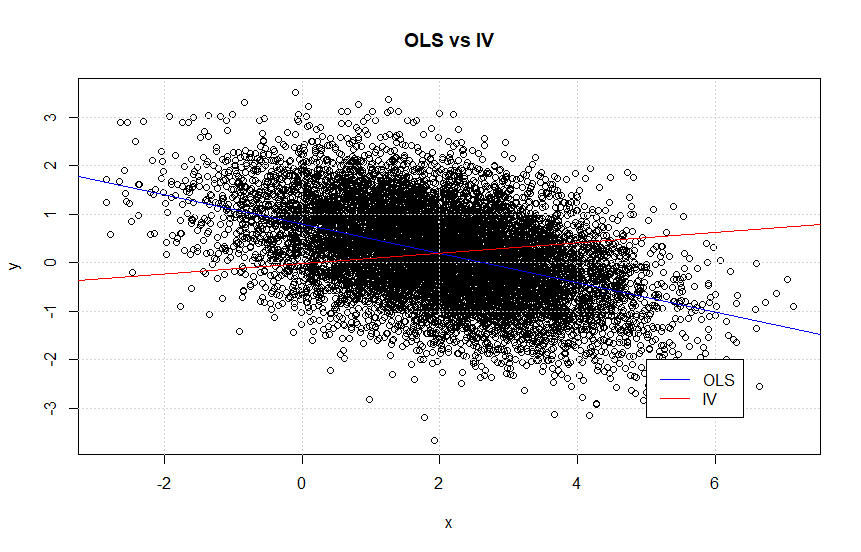
Clearly this is a situation one should be careful not to end up in.

A simple fictional example

Say that we have a company that would like to estimate the credit scores of our customers, to calculate our risk. We have an online business which means that we have limited information. Let’s say that the attribute “rockstar” has in itself a negative impact on ability to pay, however the attribute is correlated with high wages which has a positive impact on ability to pay, so the overall effect is positive. In our company we don’t care about the causal impacts, we just care about the probability that we will get paid. However, from a researchers point of view it is interesting what causal effects are driving the credit worthiness and the underlying relationship. Hence, from the comapny’s point of view an OLS model would be useful to predict the credit risk and from the researchers point of view an IV model would be considered appropriate to capture the correct causal relationship.

Conclusion

Endogeneity is a problem in academic econometrics, it distorts the interpretation of the coefficients and the explanatory power of the model. However, in practice the biased estimator still seems to capture the overall correlation direction in the normal case and from a modelling point of view it might be used for prediction (but not causal inference) with caution. But one needs to be careful about the extreme cases.

Althoug, as one of my fellow PhD student pointed out, the IV estimatior is typically used in order to get the right interpretation of the causial relationship rather than a better prediction, this is very important to emphasize. This means that the OLS estimator might still be better if one only wants to predict \(y\), but the prediction cannot directly be interpreted as causation. This can be seen from the plots “OLS vs IV” in this post, where the OLS estimate seems more in line with the data than the IV estimate.

In conclusion one should be careful about a situation in which the relationship one is trying to investigate is weak and there might be a large correlation between the regressor, \(x\) and the error term \(u\).

To end with a cliche, ‘all models are wrong…’.